First generation cars were open-topped – until motorists demanded creature comforts like protection from rain, a heater, and – later – air-conditioning. While some machine vision applications allow the camera to operate unprotected at ambient temperatures – other applications are more demanding. Components Express Inc. (CEI) provides a range of enclosures and mounts – both standard and custom – to protect your camera.
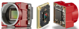
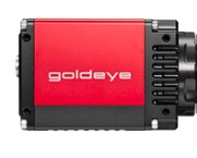
Standard enclosures may be enough for applications that don’t require wash-down, but for many applications the camera, lens, and ports need some protection. Light weight, low profile designs are available in various diameters, suitable for cameras from diverse manufacturers. Adjustable mounts with pre-tapped holes are provided. In addition to generic enclosures suitable for diverse camera models, enclosure designs are available for Teledyne Dalsa Genie Nano, Allied Vision Mako and Alvium cameras and other manufacturers.
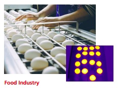
Food processing or high-particulates deployments often must be in wash-down configurations.
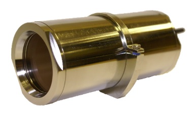
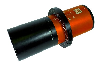
Extruded housing, with IP67 rating, features CEI Integrated Connector Design that keeps cord grips inside the housing:
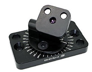
Or you may need a sturdy mount to position the camera on a stable base, with adjustable alignment options.
Custom enclosure and mounts are also available for the most demanding applications. Besides all the Components Express Inc. (CEI) mounts and enclosures, some may also be interested in air curtains, windows & filters by Midwest Optical. These also come in customer sizes, length and focusing solutions. Discuss your requirements with us!

1st Vision’s sales engineers have over 100 years of combined experience to assist in your camera and components selection. With a large portfolio of lenses, cables, NIC card and industrial computers, we can provide a full vision solution!