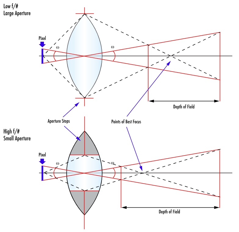
Some problems best solved outside the visible spectrum
Most of us think about vision with a human bias, since most of us are normally sighted with color stereo vision. We perceive distance, hues, shading, and intensity, for materials that emit or reflect light in the wavelengths 380 – 750 nm. Many machine vision problems can also be solved using monochrome or color light and sensors in the visible spectrum.
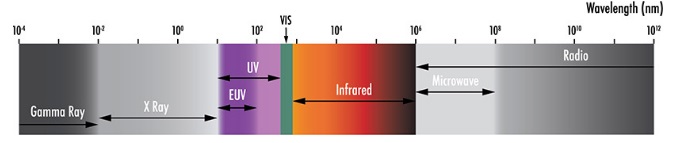
Many applications are best solved or even only solved, in wavelengths that we cannot see with our own eyes. There are sensors that react to wavelengths in these other parts of the spectrum. Particularly interesting are short wave infrared (SWIR) and ultraviolet (UV). In this blog we focus on SWIR, with wavelengths in the range 0.9 – 1.7um.
Examples in SWIR space
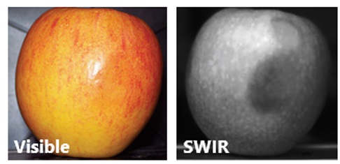
Food processing and agricultural applications possible with SWIR. Consider the above images, where the visible image shows what appears to be a ripe apple in good condition. With SWIR imaging, a significant bruise is visible – as SWIR detects higher densities of water which render as black or dark grey. Supplier yields determine profits, losses, and reputations. Apple suppliers benefit by automated sorting of apples that will travel to grocery shelves vs. lightly bruised fruit that can be profitably juiced or sauced.
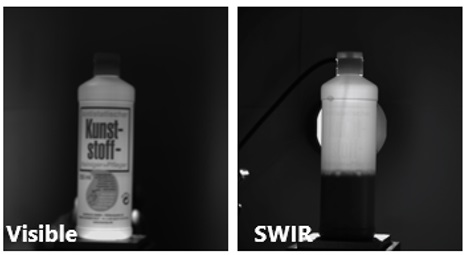
Courtesy Effilux
Whether controlling the filling apparatus or quality controlling the nominally filled bottles, SWIR light and sensors can see through glass or opaque plastic bottles and render fluids dark while air renders white. The detection side of the application is solved!
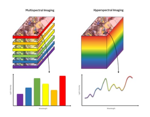
Hyperspectral imaging
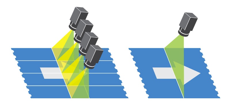
Yet another SWIR application is hyperspectral imaging. By identifying the spectral signature of every pixel in a scene, we can use light to discern the unique profile of substances. This in turn can identify the substance and permit object identification or process detection. Consider also multi-spectral imaging, an efficient sub-mode of hyperspectral imaging that only looks for certain bands sufficient to discern “all that’s needed”.
How to do SWIR imaging
The SWIR images shown above are pseudo-images, where pixel values in the SWIR spectrum have been re-mapped into the visible spectrum along grey levels. But that’s just to help our understanding, as an automated machine vision application doesn’t need to show an image to a human operator.
In machine vision, an algorithm on the host PC interprets the pixel values to identify features and make actionable determinations. Such as “move apple to juicer” or “continue filling bottle”.
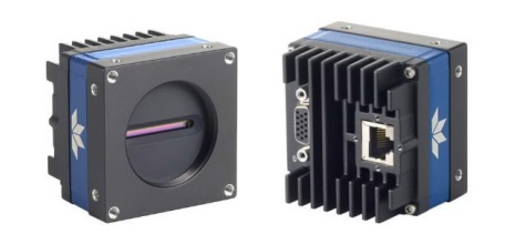
Components for SWIR imaging
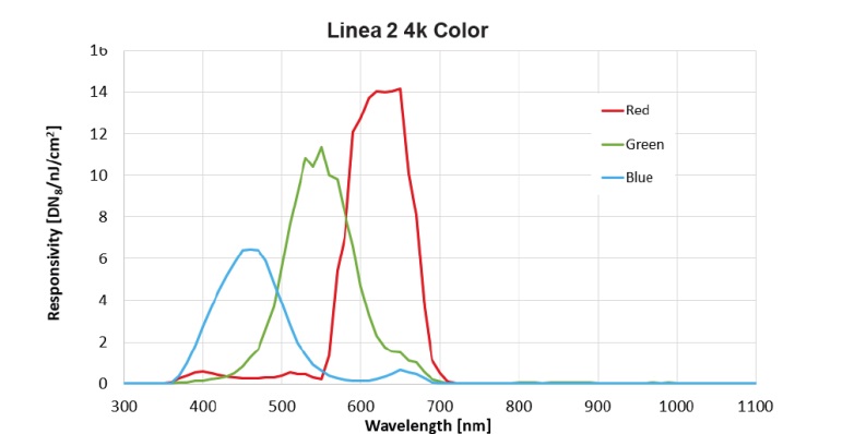
SWIR sensors and cameras; SWIR lighting, and SWIR lenses. For cameras and sensors, consider Allied Vision’s Goldeye series:
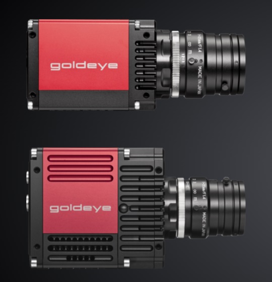
Goldeye SWIR cameras are available in compact, rugged, industrial models, or as advanced scientific versions. The former has optional thermal electric cooling (TEC), while the latter is only available in cooled versions.

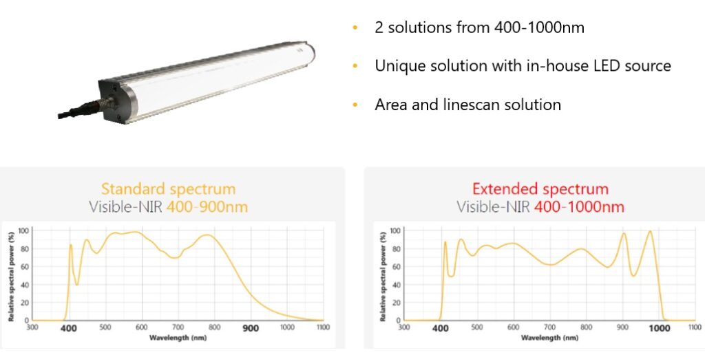
For SWIR lighting, consider Effilux bar and ring lights. Effilux lights come in various wavelengths for both the visible and SWIR applications. Contact us to discuss SWIR lighting options.

By emitting light in the SWIR range, directed to reflect off targets known to reveal features in the SWIR spectrum, one builds the components necessary for a successful application.
And don’t forget the lens. One may also need a SWIR-specific lens, or a hybrid machine vision lens that passes both visible and SWIR wavelengths. Consider Computar VISWIR Lite Series Lenses or their VISWIR Hyper-APO Series Lenses. It’s beyond the scope of this short blog to go into SWIR lensing. Read our recent blog on Wide Band SWIR Lensing and Applications or speak with your lensing professional to be sure you get the right lens.
Takeaway
Whether SWIR or UV (more on that another time), the key point is that some machine vision problems are best solved outside the human visible portions of the spectrum. While there are innovative users and manufacturers continuing to push the boundaries – these areas are sufficiently mature that solutions are predictably creatable. Think beyond the visible constraints!
Call us at 978-474-0044. Or follow the contact us link below to provide your information, and we’ll call you.

1st Vision’s sales engineers have over 100 years of combined experience to assist in your camera and components selection. With a large portfolio of lenses, cables, NIC cards and industrial computers, we can provide a full vision solution!