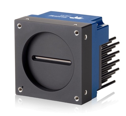
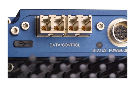
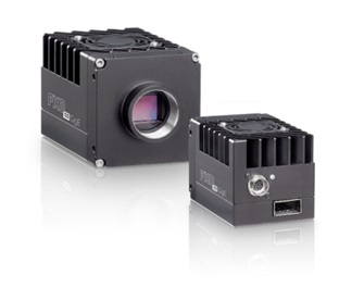
Allied Vision FXO cameras are high-speed industrial GigE Vision cameras available with 10GigE, 25GigE, and 100GigE interfaces. Built around Sony Pregius S global shutter sensors, FXO cameras deliver high image quality, fast frame rates, low-latency image transfer, and reliable performance for demanding machine vision applications.
Stable data for high-throughput metrology, semiconductor and industrial inspection
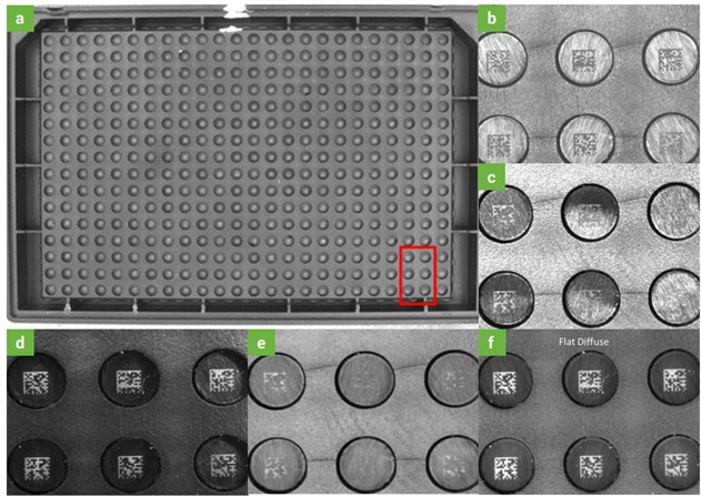
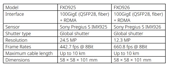
In semiconductor and electronics manufacturing, the FXO 100GigE cameras are suited for high-throughput 2D and 3D automated optical inspection because the global shutter supports fast motion without distortion and RDMA-based transport keeps data movement consistent under heavy loads.
In addition to metrology and industrial inspection, the FXO cameras are ideal for laser triangulation, 3D scanning and high-speed acquisition.
10, 25 and 100GigE FXO cameras
While the 100GigE models are the newest to join the product family, your application’s demands might be satisfied with 10GigE or 25GigE models. Even “just” the 10GigE models offer frame rates from 30 – 217fps, depending on sensor. Likewise the 25GigE models span 96 – 671fps. You wouldn’t be fishing in this pond unless framerate was a factor, but as with any engineering challenge, it’s the overall solution and fit that matters.

RDMA note
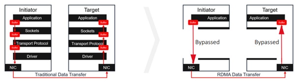
RDMA (Remote Direct Memory Access) enables the host PC to directly access camera memory, avoiding memory copy to readout buffers, operating system overhead (time) costs, or CPU load. Special network adapters are required to support RDMA. But for demanding applications, where sustained high framerates are required, without missing data, RDMA can provide low-latency throughput.
Within the FXO family, all the 100GigE cameras support RDMA, and selected models of the 25GigE cameras offer RDMA. It’s not needed on the 10GigE models.
We have a blog on RDMA if you want to dive a bit deeper on your own.
About those network adapters
Unless you are new to machine vision, you already have some experience with network adapters aka NICs or network interface controller (or cards). They come in various flavors, according to PC host bus architecture, port count, protocol, bandwidth capacity, and budget.
For the Allied Vision FXO cameras, see suggested NICs according to camera model and throughput:
- 10GigE Dual port POE PCIe NIC card
- 25GigE 2-port SFP28 Interface Card for 25GigE
- 100GigE 2-port SFP28 Interface Card for 100 GigE
Plus a pair of transceivers
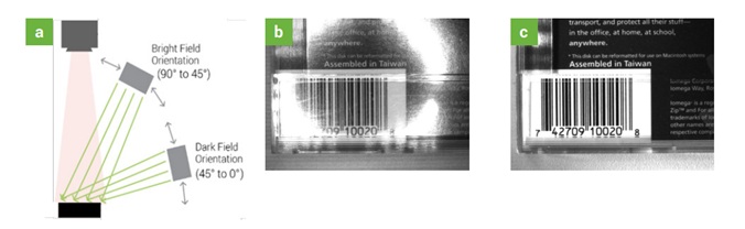
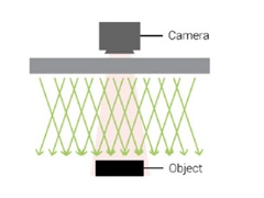
When using an RDMA camera model with fiber optic cable, you’ll also need a transceiver at both the camera and the PC host:
Transceiver: QFSP28 – you need on for each end, per diagram above
FXO camera highlights
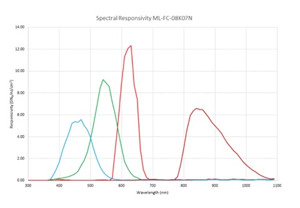
Sony Pregius S sensors – Yes we mentioned it already above, but it bears repeating. These backlit sensors are highly sensitive, low noise, and with small pixel sizes.
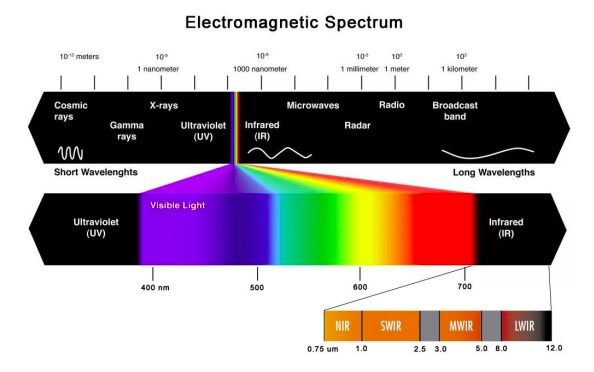
Color, monochrome, and SWIR model options – while it’s common to find the color/mono options in the same product line, the SWIR option is rather distinctive. It creates potential efficiencies for multi-spectral applications.
Long cable runs to multi-kilometer distances – QSFP28 (Quad Small Form-factor Pluggable) interface enables distances up to multiple kilometers between your PC host and the camera, via fiber.
Advanced thermal design – dissipates heat effectively to maintain low noise high-quality images.
Does your application require 25 or 100 GigE bandwidth to sustain your target image sizes and framerates? Start with application requirements and work back to sensor, camera, interface, cabling, etc. We’re here to help.

1st Vision’s sales engineers have over 100 years of combined experience to assist in your camera and components selection. With a large portfolio of cameras, lenses, cables, NIC cards and industrial computers, we can provide a full vision solution!
About you: We want to hear from you! We’ve built our brand on our know-how and like to educate the marketplace on imaging technology topics… What would you like to hear about?… Drop a line to info@1stvision.com with what topics you’d like to know more about.
#AlliedVision
#FXO
#100GigE
#Machinevision