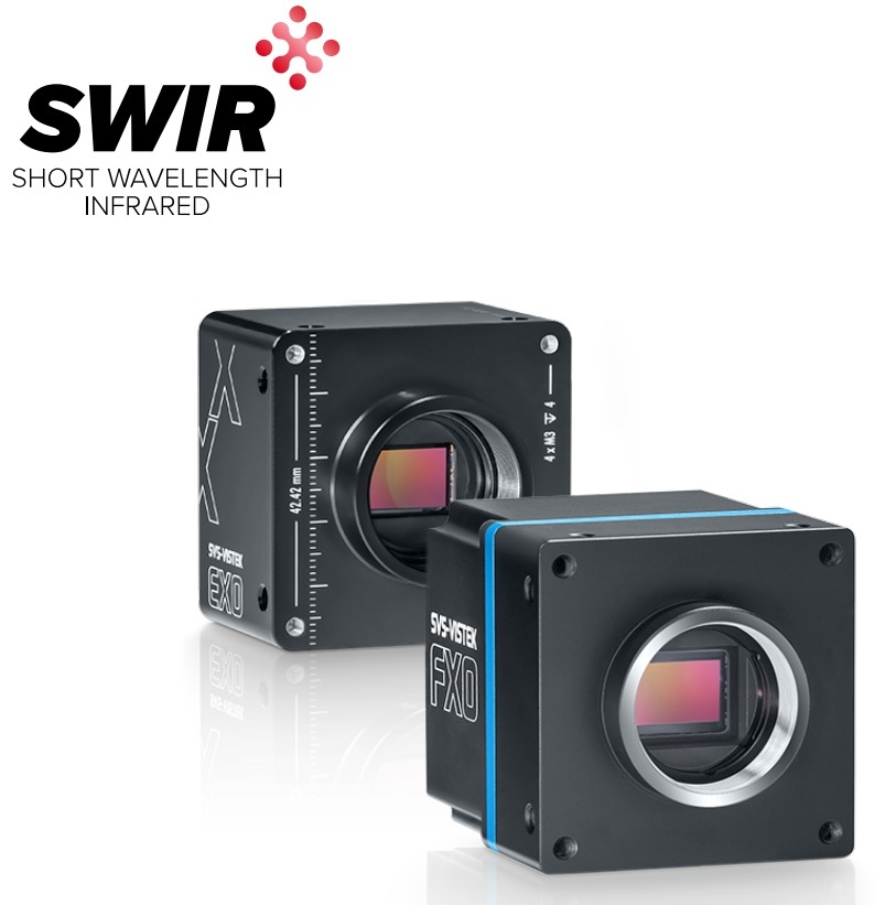
Short Wave Infrared (SWIR) imaging is enjoying double-digit growth rates, thanks to improving technologies and performance, and innovative applications. Unlike visible-light sensors, SWIR cameras can image through silicon, plastics, and other semitransparent materials. That’s really effective for many quality control applications, materials sorting and inspection, crop management, fruit sorting, medical applications, and more.
Unlike CMOS sensors, from which high-quality images are reliably derived under wide operating conditions, SWIR sensors typically need “tuning” relative to temperature and exposure duration. First generation SWIR cameras sometimes generated images that while useful, were a bit rough and with certain limitations in the extreme. SWIR camera manufacturers have been innovating solutions to raise the performance of their cameras.
What’s the problem?
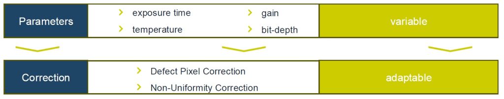
In short-wave infrared (SWIR) imaging applications, camera operation points such as exposure time, gain and bit-depth need to be adapted depending on the inspection task at hand. Image sensor defects such as defective pixels and image non-uniformities – inherent to SWIR sensors – are sensitive to the aforementioned operations points.
Unless controlled, image quality can suffer
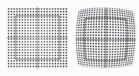
Consider the following image:
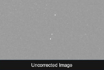
The gray field is intentionally unexciting as a flat field baseline without a target. The white dots are undesired defect pixels, an unfortunate characteristic that one can thankfully correct through interpolation. This image is meant to show “what we do NOT want”.
The four parameters exposure setting, temperature, bit-depth, and gain may collectively be called the “Operating Point” of a SWIR sensor, as together they have a significant bearing on image quality. Through manual or automated adjustments, one can optimize image outcomes.
In this blog, we provide context for these concepts. And we introduce Dynamic Operating Point Optimization (DOPO) as an automated innovation available in the fx series of SWIR cameras offered by SVS Vistek / Allied Vision.
Before Dynamic Operating Point Optimization (DOPO)
SWIR cameras with some image correction capabilities – prior to DOPO we’ll describe in the next section – certainly improved image quality. Largely via defect pixel correction (DPC) and non-uniformity correction (NUC).
Defect pixel correction (DPC) is achieved by replacing the “hot” or “dead” pixel value by the average value of its nearest neighbors. As long as there isn’t a cluster defect with multiple adjacent defect pixels (typically identified and rejected at manufacturing quality control), this is an effective solution.
Non-uniformity correction (NUC) is a bit more complex, but worth understanding. The non-uniformities arise in thermal imaging due to variations in sensitivity among pixels. If uncorrected, the target image could be negatively impacted with striations, ghost images, flecks, etc.
Factory configuration of each camera, before finalizing testing and shipping, adapts for the nuanced differences among individual sensors. Correction tables are created and stored onboard the camera, so that the user receives a camera that already compensates for the variations.
In reality it’s a bit more complicated
In fact defect pixels aren’t always simply hot or dead: they may appear only at certain operating points (exposure duration, temperature, gain, bit-depth, or combinations thereof).
Likewise for non-uniformity characteristics.
So that factory configuration mentioned above, while satisfactory for many applications, is a one size fits all best hope compromise, relative to the tools (then) available to the camera manufacturer and the price point the market would accept. Just as with t-shirts and socks, one size doesn’t really fit every need.
Dynamic Operating Point Optimization (DOPO)
Allied Vision has introduced dynamic operating point optimization (DOPO) to further automate SWIR cameras’ capacity to adapt to changes brought about by exposure time, temperature, gain, and bit depth. Let’s examine the graphic below to understand DOPO and the added value it delivers.
First consider the Y-axis, “Image Quality”. Looking at the flat-field gray block, clearly one would prefer the artifact-free characteristics of the upper region.
Also note the X-axis, “Sensor Temperature / Exposure Time”, for an uncooled thermal sensor. (Note that some thermal cameras do have sensor cooling options, but that’s a topic for another blog.) See the black line “No correction” sloping from upper left to lower right, and how the number of image artifacts grows markedly with exposure time. Without correction the defect pixels and sensor non-uniformities are very apparent.
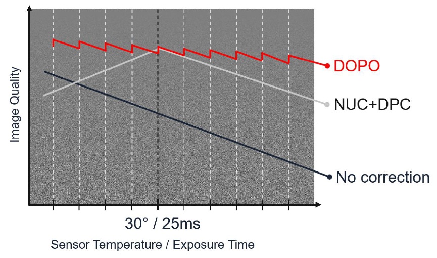
Now look at the gray lines labeled “NUC+DPC”. For a factory calibrated camera optimized for a sensor at 30 degrees Celsius and a 25ms exposure, the NUC and DPC corrections indeed optimize the image effectively – right at that particular operating point. And it’s “not bad” for exposure times of 20ms or 15ms to the left, or 30ms or 35ms to the right. But the corrections are less effective the further one gets away from that calibration point.
Finally let’s look at the zig-zag red lines labeled “DOPO”. Instead of the “one size best-guess” factory calibration, represented by the grey lines, a DOPO equipped camera is factory calibrated at up to 600 correction maps, varying each of exposure time, temperature, gain and bit depth across a range of steps, and building maps that represent all the stepwise permutations.
Takeaway: DOPO provides a set of correction tables not just one
So with DOPO providing a set of correction tables, the camera can automatically apply the best-fit correction for whatever operating point is in use. That’s the key point of DOPO. Unlike single-fit correction tables, with so many calibrated corrections under DOPO, the best-fit isn’t far off.

Thermal imaging with SWIR cameras – plenty of choices
There are a number of options as one selects a SWIR camera. Is your choice driven mostly by performance under extreme conditions? Size? Cost? A combination of these?
Call us at 978-474-0044. We can guide you to a best-fit solution, according to your requirements.
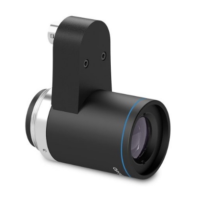
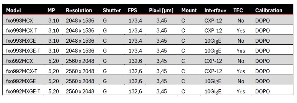
We might recommend a DOPO equipped camera, such as one of the fxo series SWIR cameras:
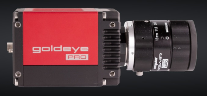
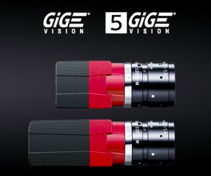
Or you might be best-served with a Goldeye camera, in cooled or uncooled models:
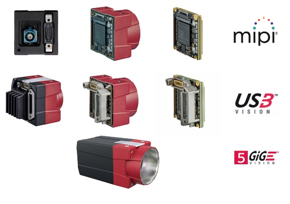
Or an Alvium compact camera, whether housed or modular (for embedded designs), in USB / MIPI CSI-2 or GigE interfaces.
The key message of this blog is to introduce Dynamic Operating Point Optimization – DOPO – as a set of factory calibration tables and the camera’s ability to switch amongst them. An equally important takeaway is that you may or may not need DOPO for a particular thermal imaging application. There are many SWIR options, in cameras and lenses, and we can help you choose.

1st Vision’s sales engineers have over 100 years of combined experience to assist in your camera and components selection. With a large portfolio of cameras, lenses, cables, NIC cards and industrial computers, we can provide a full vision solution!
About you: We want to hear from you! We’ve built our brand on our know-how and like to educate the marketplace on imaging technology topics… What would you like to hear about?… Drop a line to info@1stvision.com with what topics you’d like to know more about.